This section covers tuning the velocity and position loops in the AKD. Servo tuning is the process of setting the various drive coefficients that are needed for the drive to optimally control the servo motor for your application. There are different ways to tune, and several are covered here. We will give you guidance on what the different methods of tuning are and when to use them.
The AKD works in three major operation modes: torqueTorque is the tendency of a force to rotate an object about an axis. Just as a force is a push or a pull, a torque can be thought of as a twist, velocity, and position operation mode. No servo loop tuning is required for torque mode. Velocity loop and position loop tuning are covered below.
The AKD has an auto tuner that will provide the tuning that many applications will need. This section describes the tuning process and how to tune the AKD, specifically for cases where the user does not want to use the auto tuner.
Tuning in this section will focus on tuning in the time domain. This means that we will look at the velocity or position response vs. time as the criteria we use to decide how well tuned a control loop is tuned.
Choosing the proper specifications for a machine is a prerequisite for tuning. Unless you have a clear understanding of the type of performance needed to push the machine into production, the tuning process will cause more problems and headaches than it solves. Take time to layout ALL the requirements of the machine—nothing is too trivial to consider.
- +/– x position error counts during the entire motion.
- Settling within +/- x position error counts, within y milliseconds.
- Velocity tolerance of x% measured over y samples.
After you have constructed a detailed servo performance specification, you are now ready to start tuning your system.
In the worst case, if something goes wrong during tuning, the servo can run away violently. You need to make sure that the system is capable of safely dealing with a servo run away. The drive has several features that can make a servo run away safer:
The closed loop control loop is responsible for the desired position and / or velocity (trajectory) of the motor and commanding the appropriate current to the motor to achieve that trajectory. The challenge in closed loop control loops is to make a system that not only follows the desired trajectory, but also is stable in all conditions and resist external forces, and do all of this at the same time.
When in velocity operation mode, only the velocity loop is tuned. When in position operation mode, both the velocity and position loops must be tuned.
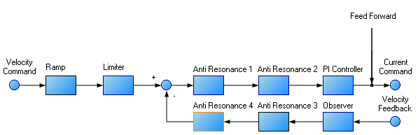
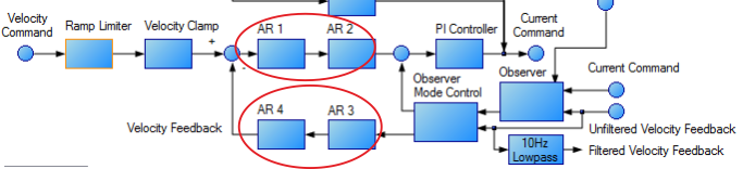
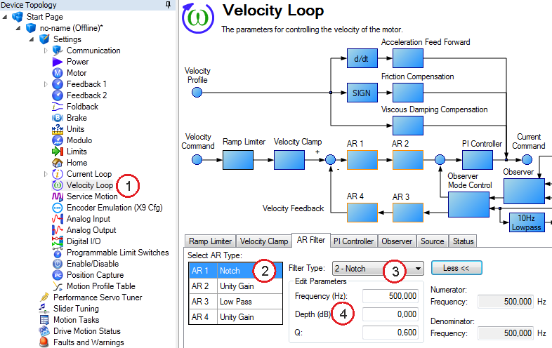
The velocity loop on the AKD consists of a PI (proportional, integral) in series with two anti-resonance filters (ARF) in the forward path and two-anti resonance filters in series in the feedback path.
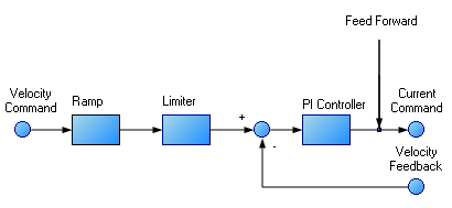
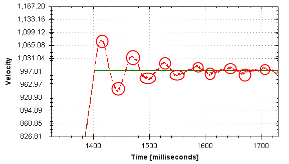
To perform basic tuning of the velocity loop, you can use just the PI block and set ARF1 and ARF2 to unity (no effect) and set the observer to 0 (no effect). Using just the PI block simplifies the process of tuning the velocity loop. To start tuning you can adjust the PI Controller block first. A simplified velocity loop without anti-resonant filters and observer is shown below. This is how you can think of the loop before the anti resonant filters and observer is used.
Procedure for simple velocity loop tuning:
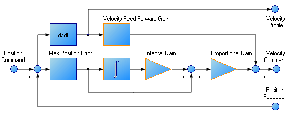
The position loop is a second loop that builds upon a correctly tuned velocity loop to provide accurate control over position. The position loop is a simple element that consists of a PI loop. It is simplest to tune the P and I terms in the velocity loop and use only the P term in the position loop.
At most, use only three non-zero P and I terms from both the velocity loop and the position loop. One combination would be VL.KP, VL.KI, and PL.KP. Another valid combination would be VL.KP, PL.KP, and PL.KI. The VL.KP, VL.KI, and PL.KP combination is shown here.
Procedure for tuning position loop:
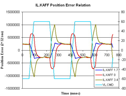
The torque based feedforward terms on the AKD effectively model the physics of your motor and allow the drive to command the appropriate current, even before the encoder has time to send data back to the drive. TorqueTorque is the tendency of a force to rotate an object about an axis. Just as a force is a push or a pull, a torque can be thought of as a twist based feedforward terms allow you to lower following error with virtually no stability penalty.
To adjust IL"Instruction list" This is a low-level language and resembles assembly.KAFF:
The AKD has four anti-resonance filters. Two filters are in the forward path and two are in the feedback path.
Similarities
Differences
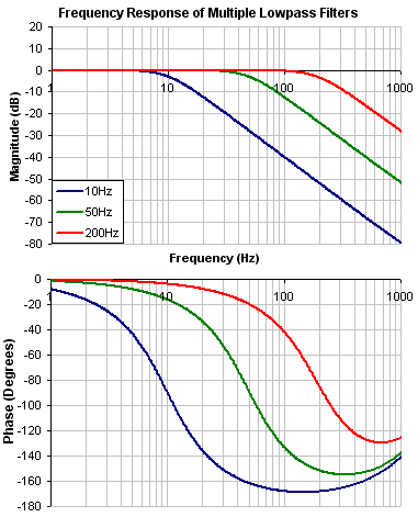
Low Pass
A low pass filter allows signals through below a corner frequency and attenuates the signals above the same corner frequency. The behavior at the corner frequency can be specified with the low-spass Q.
To specify a lowpass filter, you must specify the frequency and Q for both the zero and pole on anti-resonance filter 1. To do this, see the following example using the terminal commands that sets:
VL.ARTYPE1 0
VL.ARZF1 700
VL.ARZQ1 0.707
VL.ARPF1 5000
VL.ARPQ1 0.707
Lead Lag
A lead lag filter is a filter that has 0 dB gain at low frequencies and a gain that you specify at high frequencies. You also specify the frequency that the gain at which the transition occurs.
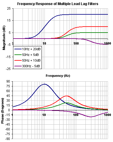
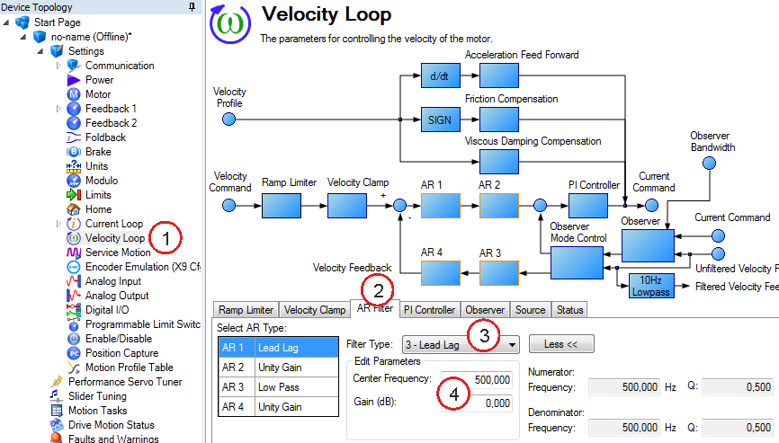
To specify a Lead Lag filter, you must specify the Center Frequency and high frequency Gain (dB). To do this, see the following example by clicking on the Velocity Loop:
Click on Velocity Loop
Notch
A notch filter changes gain at a specific frequency. You specify the frequency at which the gain change occurs (Frequency (Hz)), how wide of a frequency range the cut occurs (Q), and how much the gain changes (Notch Depth (dB)).
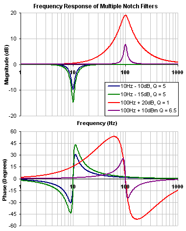
To specify a notch filter, you must specify the Frequency (Hz), Depth (dB) and Width (Q) of the notch. To do this, see the following example by clicking on the Velocity Loop:
Click on Velocity Loop (1), then select the AR1 Tab (2), using the Filter Type drop-down, select Notch (3), lastly, enter the desired Frequency, Depth and Q of the Notch filter (4).
Biquad
A biquad is a flexible filter that can be thought up as being made up of two simpler filters; a zero (numerator) and a pole (denominator). In fact, the pre-defined filters mentioned above are really just special cases of the biquad.
Both the zero (numerator) and the pole (denominator) have a flat frequency response at low frequencies and a rising frequency response at high frequencies. The transition frequency and damping must be specified for both the numerator and denominator.
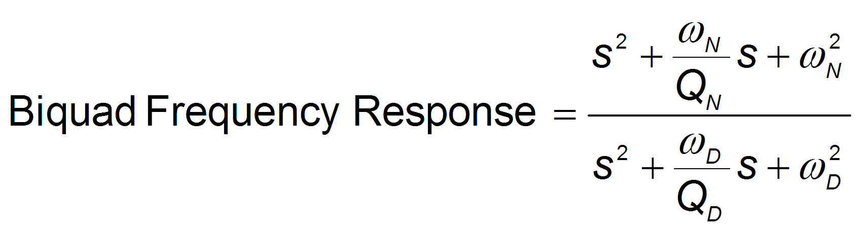
Analyzing the numerator and denominator, the frequency response calculation is simple:
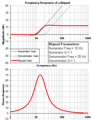
If the numerator and denominator are plotted in dB, the biquad response is numerator – denominator. Understanding how the numerator and denominator work is crucial in understanding how a biquad frequency response is created.
Below is an example of a biquad filter similar to a Lead Lag filter type. To help understand how to determine the frequency response of the biquad, the numerator and denominator response have been plotted. If the denominator is subtracted from the numerator, the biquad response is the result.
The biquad filter is very flexible, which allows custom filters to be designed. Below is an example of a resonance filter using a biquad. Notice how the high Q values affect the numerator and denominator. This gives a biquad frequency response similar to a mechanical resonance.
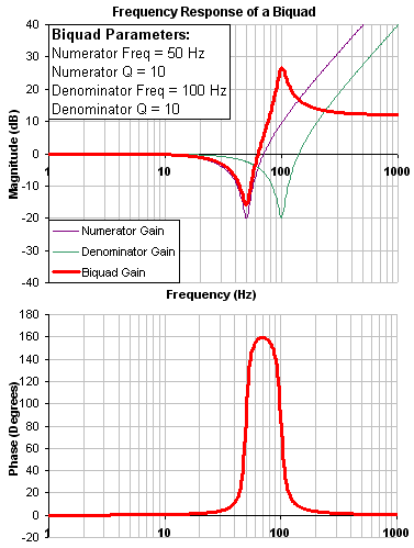
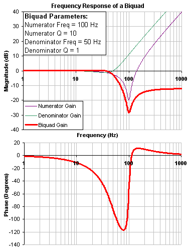
The previous two examples used a numerator frequency lower than the denominator frequency, yielding a positive gain in high frequencies. If the denominator frequency is lower than the numerator frequency, then high frequencies will have a negative gain.
Below is an example where the numerator frequency is higher than the denominator. Notice the high frequencies have a negative gain.
To specify a biquad filter, you must specify the frequency and Q for both the zero and the pole on anti-resonance filter 3. To do this, see the following example using the terminal commands that sets:
VL.ARTYPE3 0
VL.ARZF3 100
VL.ARZQ3 0.7
VL.ARPF3 1000
VL.ARPQ3 0.8
In the s-domain, the linear biquad response is calculated:
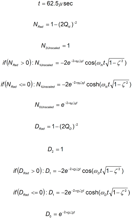
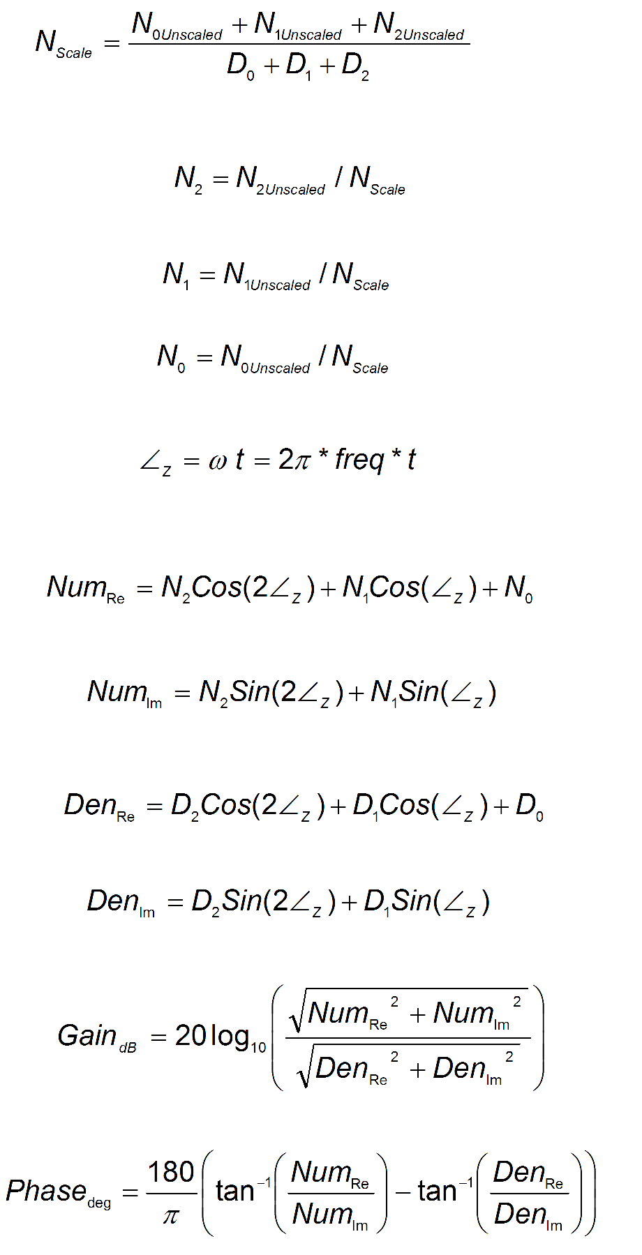
To convert from idealized s-domain behavior to a more realistic z-domain behavior, we convert using a pole / zero transform. To calculate the frequency response for an individual frequency:
Low pass filters in the feedback path. This is a common way to deal with noisy feedback sensors. When used in combination with noisy feedback sensors, significant reduction in audible noise can result.
Lead / lag filters in the forward path. This is a common way to achieve phase lead for control loops without exciting high frequency resonances.
Low pass filters in the forward path. This is a common way to limit high frequency energy from reaching a system that can not productively use energy at these high frequencies. This is also used to lower the effect of system resonances over a wide range of frequencies.
Notch filters are used to cancel system resonances. Notch filters are designed to be the opposite in amplitude of system resonances. Notch filters are applied to very specific frequencies, and therefore you must know your system resonance frequencies accurately to use them effectively.
|
Stay Connected with Kollmorgen       
|
Copyright © 2015 Kollmorgen™ |

|